- Optic Flow
WHAT IS OPTIC FLOW?
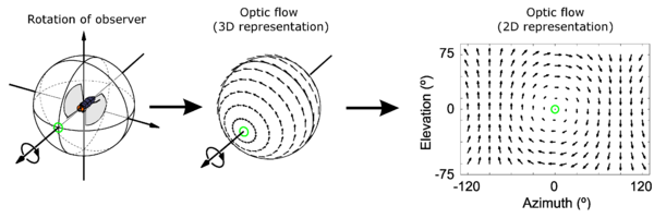
Optical flow or optic flow is the pattern of apparetn motion of objects, surfaces, and edges in a visual scene caused by the relative motion between an observer and the scene. Optical flow techniques such as motion detection, object segmentation, time-to-collision and focus of expansion calculations, motion compensated encoding, and stereo disparity measurement utilized this motion of the objects surfaces, and edges.
http://en.wikipedia.org/wiki/Optical_flow
ESTIMATION OF THE OPTIAL FLOW
Sequences of ordered Images allow the estimation of motion as either instantaneous image velocities or discrete image displacements.
The optical flow methods try to calculate the motion between two image frames which are taken at times t and t + δt at every voxel position. These methods are called differential since they are based on local Taylor series approximations of the image signal; that is, they use partial derivatives with respect to the spatial and temporal coordinates.
For a 2D+t dimensional case (3D or n-D cases are similar) a voxel at location (x,y,t) with intensity I(x,y,t) will have moved by δx, δy and δt between the two image frames, and the following image constraint equation can be given:
I
(x,y,t) = I(x + δx,y + δy,t + δt)
Assuming the movement to be small, the image constraint at I(x,y,t) with Talor series can be developed to get

where H.O.T mean higer order terms, which are small enough to be ignored. From these equations it follow that:
or
which results in
where Vx, Vy are the x and y components of the velocity or optical flow of I(x,y,t) and
 and
and  are the derivatives of the image at (x,y,t) in the correspoing directions Ix,Iy and It can be wirtten for the drivatives in the following
Thus
IxVx +
IyVy = - It
This is an equation in two unknowns and cannot be solved as such. This is known as the aperture proble of the optical flow algorithm.
OPTIC FLOW APPLICATION(MATLAB)
◆Obstacle Avoidance
In robotics, obstacle avoidance is the task of satisfying some control objective subject to onon-intersection or noncollision position constraints. To avoid arbitrary obstacles in an unknown environoment, the accrutate sensingis required. Normally the sonar, light or tactile sensor is used for localization. Sonar ranging is one of the most common forms of distance measurement used in mobile robots and a variety of applications. Although Sonar ranging sensor is most used method, I suggest a new method for obstacle avoidance based on optic flow method. The picture below shows successive process of finding a direction to avoid obstacles. Figure1 (A) displays optical flow arrows when a mobile robot heads toward obstacles. The arrow lean towrad the direction awya from the robot.

Figure1
Technically, optical flow is being generated based on a grid; a series of optic flow, so to speak, is on the same horizontal line. Picture (B), horizontal arrow represent  components; the closer the object is, the larger the magnitude of optic flow arrow is. As shown in Figure below, normally, the optic flows are randomly distributed on a horizontal line: right direction compoments(
 ) and left direction components (
 ). In order to rearrange and resize thses components, equatino (1) proposes simple method.
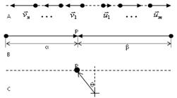
Figure2
 ,
,  ..........(1)
The point P represents the proportional point which each  and
and  occupies. In Figure 2(B), the size of
  is bigger than the size of
  . This means the obstacle at the right side is closer than the left one. Thus, the line from the origin to the point P, in Figure 2(C), has angular deviation
  to the left. The angle
 can be found for every single horizontal line in the grid. The mean value of the angle
 , in Figure1(D), represents the final vector the robot has to head towards.
Figure3
◆Rotating Angle
Unlike wheel based mobile robots, the posture control is needed for legged robots. Crab's eyes set the orientation to the equator line in their territorial field. Crab's special visual system may have influences on the stabillization of the robot body.
Here, I propose that the stabilizatioin control problem can be solved using optical flow. Although the posture control is being limited to the 2-dimension space, this method is simple and effective.
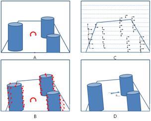
Figure4
As shown in Figure4(B), the camera on the mobile robot is tilted due to the motion of the robot. The optical flow arrows always lean towards the opposite direction of the viewer's progression direction. The scene in the pircure is rotated counterclockwise, and the optical flow arrows head clockwise. The optic flow method is based on the pixel movements. Consequently, the pixels, away from the center of the rotation, make more movements than those pixels close to the center. Since The pixel movement makes optic flows, large pixel movement makes big magnitude of optic flow. In the same manner, in Figure 4(B), optic flow arrows away from center are bigger than the centerd one. In order to calculate the angle of the optic flow, in Figure 4(C), each optical flow arrow is divided into (x,y) vector components. The angle of each optic flow is based on the horizontal line in the picture. The angle can be calculated from equation(2).
 .................(2)
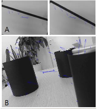
Figure5
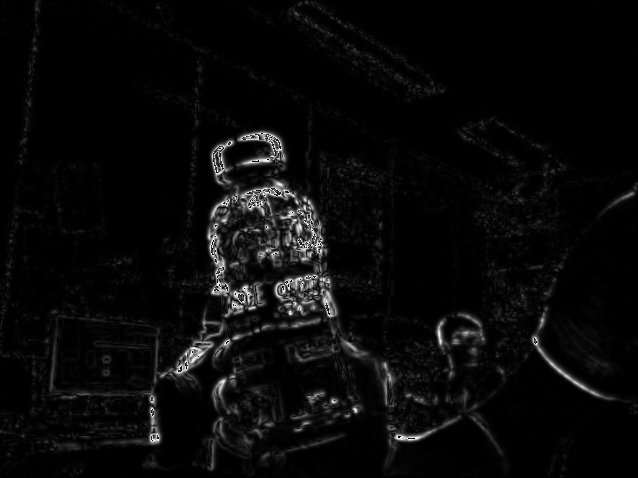
TEST
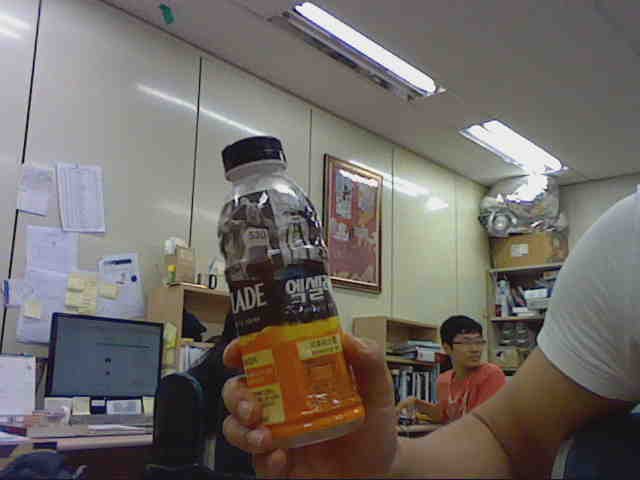
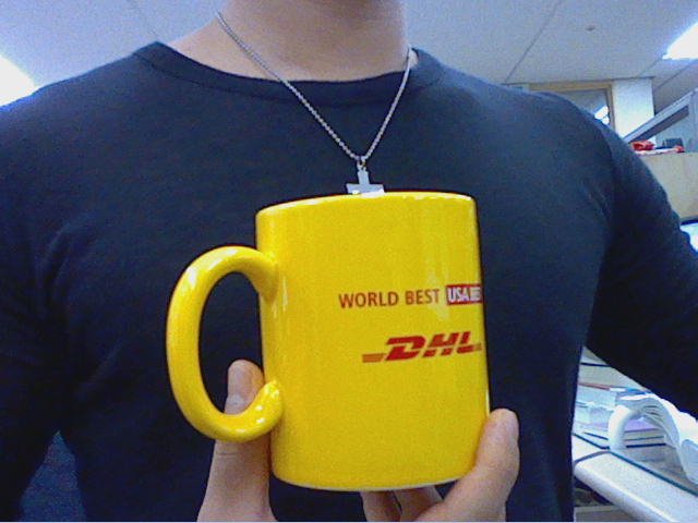
Optici flow needs two consecutive pictures to process. In C language, there is no convenient way to draw arrows, a intensity of color is being substituted for the magnitude of arrows.
|
|
|
 |
 |
 |
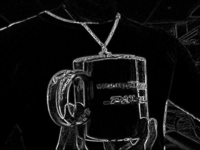 |
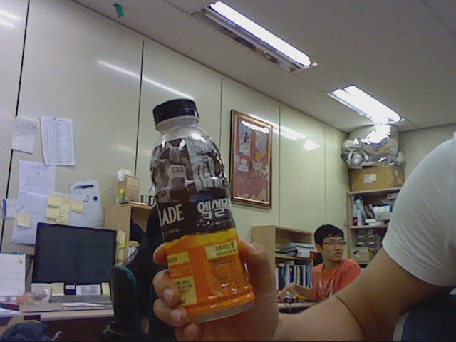
As I shake the bottle and cup, the movement of pixels around the bottle and cup are greater than other pixels in background. This represents high intensity of white color around the bottle.
 |
 |
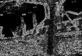 |
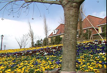
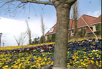
Two consecutive pictures of a landscape. Those two pictures are taken in the moving car, so the pixels in the picture are being shifted to the same direction.